Lets Tutorial

Reading AMSR 2 Data into GeoTIFF raster using gdal grid

The passive microwave data from the Advanced Microwave Scanning Radiometer (AMSR), available at https://gcom-w1.jaxa.jp/auth.html, is delivered in orbital swaths. The raster band contain the image data in various frequency range, and the geolocation information for 89GHz is stored in one containing latitude values for each pixel, and another channel containing longitude values for each pixel. This data needs processing before having a regular geocoded raster.

The following is not an exhaustive description, but extended notes on how to read AMSR-2 files, which possibly may be of   help to others trying to solve a similar task.

For some, the final commented script at our github page may be enough help, the text below tries to explain the most important steps in this script:

The various frequency bands of AMSR-2 have different resolution (see the product specs and the user manual ), we choose the L1R dataset, where the data is already processed to match the geolocation stored in the lat/long band for 89GHz.

Information on the hdf image can be retrieved with gdalinfo:

gdalinfo C:UsersmaxDocumentsGW1AM2_201301311114_050A_L1SGBTBR_1110110.h5

The metadata printed out contains the names of the subchannels, as seen here:
and information about a specific channel can be retrieved by using gdalinfo on exactly this subchannel-name from the metadata:

gdalinfo HDF5:"C:UsersmaxDocumentsGW1AM2_201301311114_050A_L1SGBTBR_1110110.h5"://Brightness_Temperature_(89.0GHz-A,V)

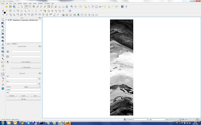
Opening one of the bands in QGIS, the data looks like this (all images in this post are © JAXA EORC ):

HDFfile = gdal.Open( rC:UsersmaxDocumentsGW1AM2_201301311114_050A_L1SGBTBR_1110110.h5 )

HDF_bands = HDFfile.GetSubDatasets()

#HDF Subdatasets are opened just as files are opened:
HDF_SubDataset = gdal.Open(HDF_bands[channel][0])
HDF_SubDataset_array = HDF_SubDataset.ReadAsArray()

HDF_Lat89A = gdal.Open(HDF_bands[46][0])
HDF_Lat89A_array = HDF_Lat89A.ReadAsArray()
 
HDF_Lon89A = gdal.Open(HDF_bands[48][0])
HDF_Lon89A_array = HDF_Lon89A.ReadAsArray()

In the next step, a create a comma-separated file containing longitude, latitude, brightness values for each raster point. This comma separated file is then the input for gdal_grid. I loop through each pixel and write the three values (  longitude, latitude, brightness ) into a csv-file.

So for the 89GHz channel, I write both 89A and 89B to a csv-file:

 
#Add header line to textfile
textfile = open( AMSRcsv, w)
textfile.write(lon,lat,brightness
)

## Loop through each pixel and write lon/lat/brightness to csv file
for i in range(rows):
    for j in range(cols):
        wgs84=pyproj.Proj("+init=EPSG:4326")
        EPSG3411=pyproj.Proj("+init=EPSG:3411")
     
        lonA = HDF_Lon89A_array[i,j]
        latA = HDF_Lat89A_array[i,j]

        # lon/lat written to file already projected to EPSG:3411
        (lonA_3411, latA_3411) = pyproj.transform(wgs84, EPSG3411, lonA, latA)
        brightnessA = HDF_Br89AH_array[i,j]* 0.01 #APPLYING SCALING FACTOR!

        lonB = HDF_Lon89B_array[i,j]
        latB = HDF_Lat89B_array[i,j]

        # lon/lat written to file already projected to EPSG:3411
        (lonB_3411, latB_3411) = pyproj.transform(wgs84, EPSG3411, lonB, latB)
        brightnessB = HDF_Br89BH_array[i,j]* 0.01 #APPLYING SCALING FACTOR!

        if 35 < latA < 90:
            textfile.write(str(lonA_3411) + , + str(latA_3411) + , + str(brightnessA) + 
)

        if 35 < latB < 90:
            textfile.write(str(lonB_3411) + , + str(latB_3411) + , + str(brightnessB) + 
)
       
textfile.close()

For the lower resolution channels, I use the odd numbers of the 89A long and lat channel:

 
#Add header line to textfile
textfile = open( AMSRcsv, w)
textfile.write(lon,lat,brightness
)

## Loop through each pixel and write lon/lat/brightness to csv file
for i in range(rows):
    for j in range(cols):
        wgs84=pyproj.Proj("+init=EPSG:4326")
        EPSG3411=pyproj.Proj("+init=EPSG:3411")

        #For low resolution the odd columns of Lon/Lat89 array to be taken!
        lonA = HDF_Lon89A_array[(i) ,(j*2+1)]
        latA = HDF_Lat89A_array[(i) ,(j*2+1)]

        # lon/lat written to file already projected to EPSG:3411
        (lonA_3411, latA_3411) = pyproj.transform(wgs84, EPSG3411, lonA, latA)
        brightnessA = HDF_SubDataset_array[i,j]* 0.01 #APPLYING SCALING FACTOR!

        if 35 < latA < 90:
            textfile.write(str(lonA_3411) + , + str(latA_3411) + , + str(brightnessA) + 
)

textfile.close()

Now I can almost run the gdal_grid, but as described at http://www.gdal.org/gdal_grid.html I need to create a xml file describing my comma-separated csv file.

 
<OGRVRTDataSource>
 <OGRVRTLayer name="GW1AM2_201301010834_032D_L1SGRTBR_1110110_channel89H">
  <SrcDataSource>G:AMSRGW1AM2_201301010834_032D_L1SGRTBR_1110110_channel89H.csv</SrcDataSource>
  <GeometryType>wkbPoint</GeometryType>
  <GeometryField encoding="PointFromColumns" x="lon" y="lat" z="brightness" />
 </OGRVRTLayer>
</OGRVRTDataSource>

This xml file above can be created in a python script in the following manner, some more info here:

root = ET.Element("OGRVRTDataSource")

OGRVRTLayer  = ET.SubElement(root, "OGRVRTLayer")
OGRVRTLayer.set("name", AMSRcsv_shortname)

SrcDataSource = ET.SubElement(OGRVRTLayer, "SrcDataSource")
SrcDataSource.text = AMSRcsv

GeometryType = ET.SubElement(OGRVRTLayer, "GeometryType")
GeometryType.text = "wkbPoint"

GeometryField = ET.SubElement(OGRVRTLayer,"GeometryField")
GeometryField.set("encoding", "PointFromColumns")

GeometryField.set("x", "lon")
GeometryField.set("y", "lat")
GeometryField.set("z", "brightness")

tree = ET.ElementTree(root)
tree.write(AMSRcsv_vrt)

Now we finally can run gdal_grid, either command line:

gdal_grid -a_srs EPSG:3411 -a average:radius1=4000:radius2=4000:min_points=1 -txe -3850000 3750000 -tye -5350000 5850000 -outsize 760 1120 -l GW1AM2_201301010834_032D_L1SGRTBR_1110110_channel89H GW1AM2_201301010834_032D_L1SGRTBR_1110110_channel89H.vrt GW1AM2_201301010834_032D_L1SGRTBR_1110110_channel89H.tif

or called from a Python script:

AMSRcsv_shortname =  GW1AM2_201301010834_032D_L1SGRTBR_1110110_channel89H
AMSRcvs_vrt = GW1AM2_201301010834_032D_L1SGRTBR_1110110_channel89H.vrt
AMSR_tif = GW1AM2_201301010834_032D_L1SGRTBR_1110110_channel89H.tif  

radius1 = 4000  
radius2 = 4000  
os.system(gdal_grid -a_srs EPSG:3411 -a average:radius1= + str(radius1) + :radius2= + str(radius2) + :min_points=1 -txe -3850000 3750000 -tye -5350000 5850000 -outsize 760 1120 -l  + AMSRcsv_shortname +    + AMSRcsv_vrt +   + AMSR_tif)

The radius indicates in which distance around a given output raster point the algorithm searches for points falling into the NSIDC raster -- if too small, it will result in empty pixels, if too large there will be too much smoothing since many pixels are averaged into one.

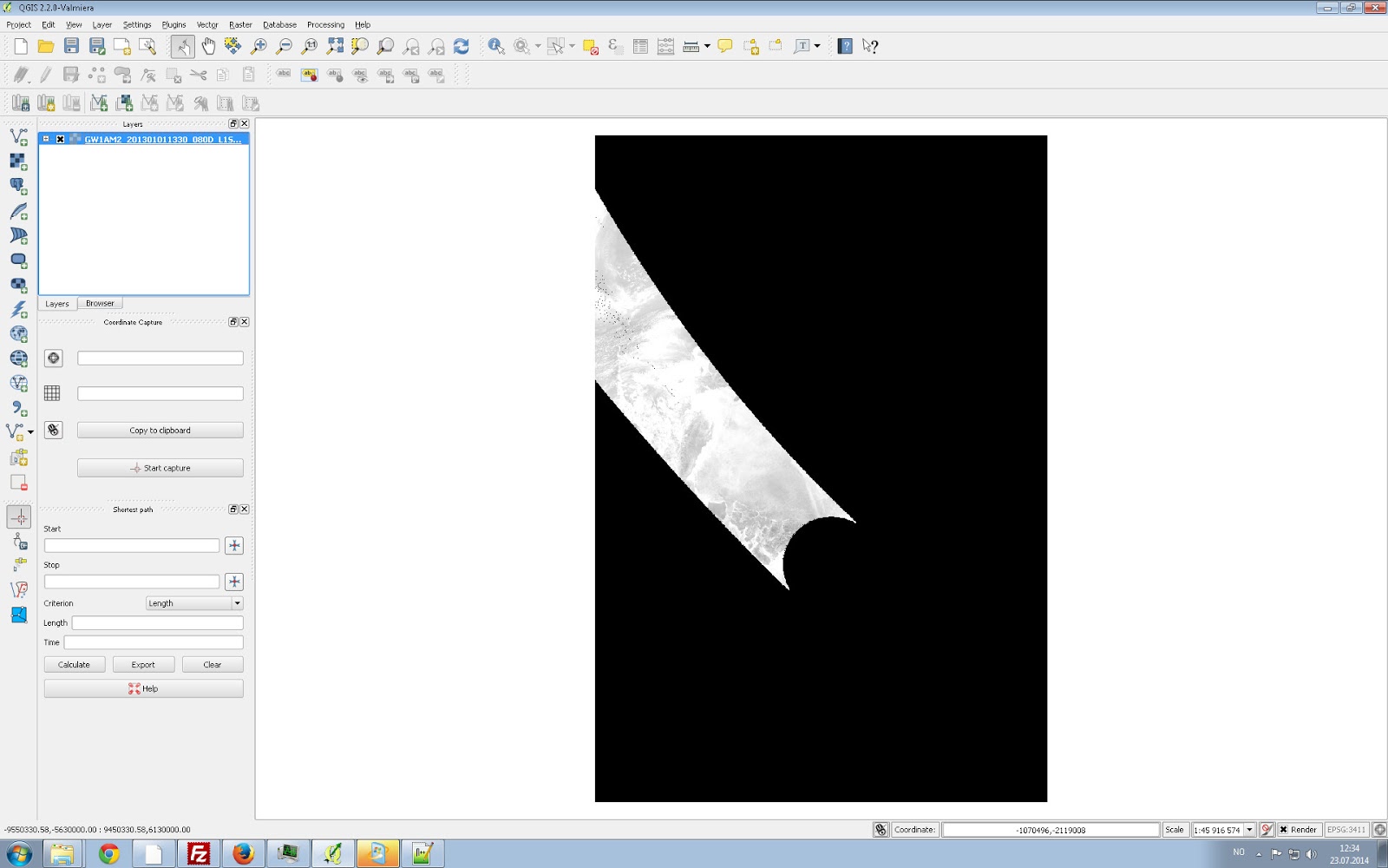
The result is, finally, the part of the swath falling into the NSIDC-raster:


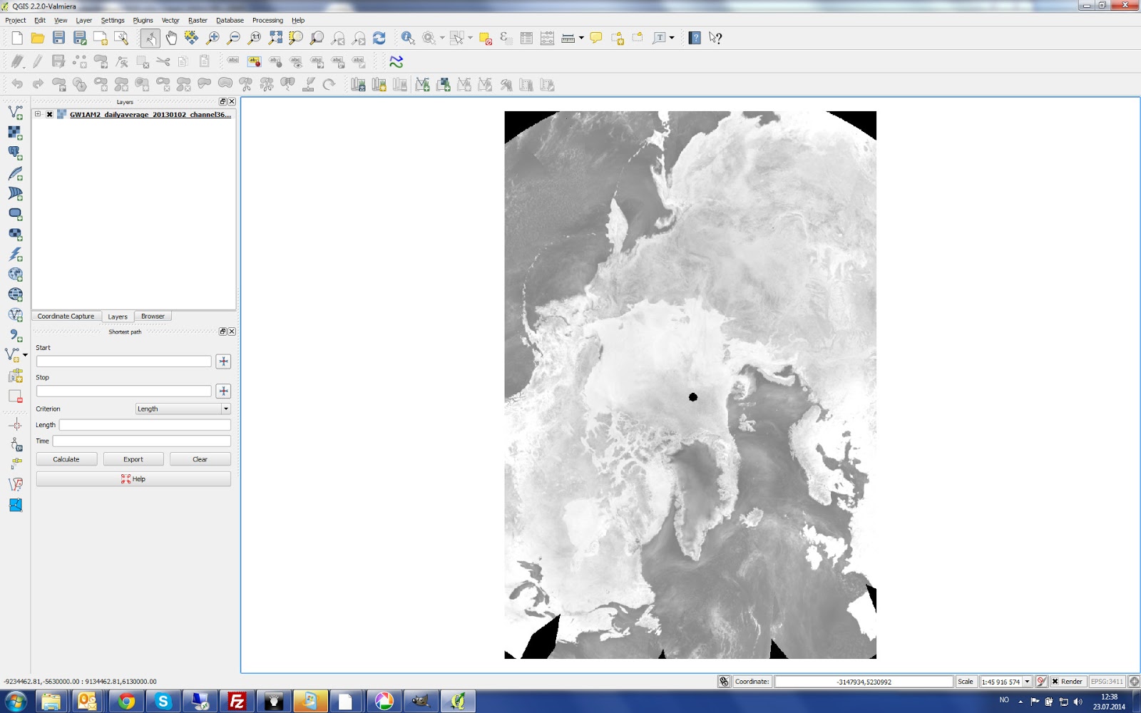
In a final step, I take all of such swaths for one day and average them into a full image of that given day, see the Average Daily function in the script for details (images  © JAXA EORC ).


One issue using gdal_grid is its very low performance regarding speed (see this comment ), one 89GHz band takes 10 minutes and a lower resolution band 2 minutes calculation time. This is then about 25 minutes for all channels of one hdf file, and since every day has about 20 files, this means 8 hours for one averaged daily raster. gdal_grid may therefore not always be feasible until the speed issue is improved.